Conditional formatting in Microsoft Excel

You may need to format certain cells like through color coding cells in Excel based on conditions using conditional formatting. In a spreadsheet, it is a great method to visualise data. Additionally, you can develop rules using your own formulas. You can find detailed explanations of the most common conditional formatting functions from the top Advanced Excel Teachers of Best Advanced Excel Institute in Dwarka

What is conditional formatting?

Microsoft Excel has a feature called conditional formatting that enables you to format your cells in a particular way depending on certain conditions. You can use it to interpret your data and identify important trends.

Highlight cells using conditional formatting

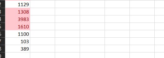
Starting off, let’s draw attention to the cells with values higher than 1209. Put these steps into action:

• Choose the range of cells to which the highlight should be applied.

• Click Conditional Formatting in the Styles Group section of the Home page.
• Highlight Cells Rules > Greater Than by clicking

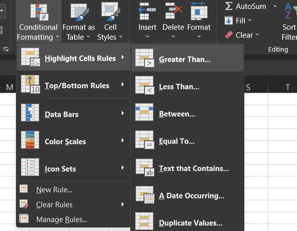
• Select the formatting style after entering the required value.

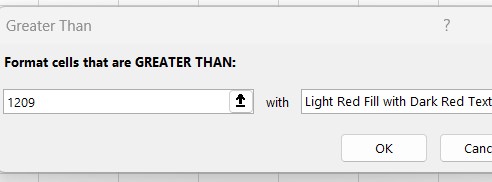
• Click OK

Clear formatting

Follow these procedures to remove the formatting guidelines

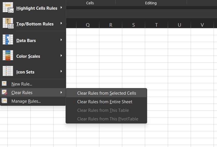
• Choose the cells in the range to which conditional formatting will be applied.
• Select the Home tab, the Styles Group, and Conditional Formatting.
• Select Clear Rules. Rules from Selected Cells are Cleared

Conditional formatting with formulas

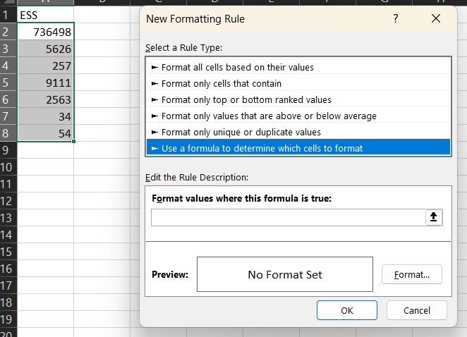
• Conditional formatting formulas must evaluate as true or false.
• Choose the cells within a range to which you want to apply conditional formatting.
• Click Conditional Formatting in the Styles Group section of the Home page.
• Select “New Rule”
• To choose which cells to format, click “Use a formula.” And put the formula in
• Click OK after choosing a formatting option.

Highlight top/bottom items

You can also retrieve the top and bottom elements in your sheet by using conditional formatting. Let’s say you want to find the five lowest from the list. Follow these instructions to do that:

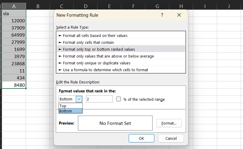
• Choose the cells within a range to which you want to apply conditional formatting.
• Click Conditional Formatting in the Styles Group section of the Home page.
• Click Bottom 10 Items > Top/Bottom Rules formatting with conditions
• Mention how many of the lowest records you want to draw attention to lowest 3
• Select OK.

Find duplicate values in the range of cell

Using conditional formatting, highlight the duplicate values in a group of cells. To put that into action, do the following:

• Choose the cell range.
• Go to the Styles Group > Conditional Formatting section on the Home tab.
• Select Duplicate values under Highlight Cells Rules.

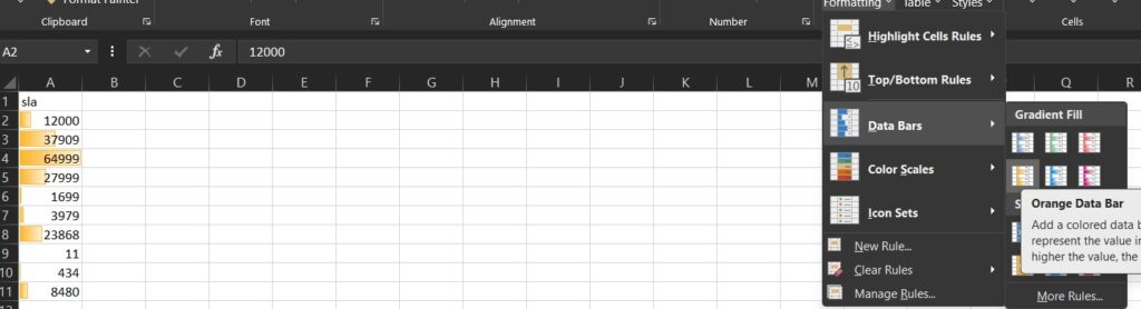
Data Bars in conditional formatting

Excel uses data bars to display the range of cells. A higher value is represented by the longer bar. Data bars are excellent tools for measuring progress as well as for comparing data to one another. Follow these procedures to add the data bars:

• Choose the cell range.
• Select a subtype under Conditional Formatting > Data Bars on the Home tab

Colour scales in conditional formatting

Excel’s colour scales make it simple to see the numbers in a group of cells. The steps below can be used to add a colour scale:

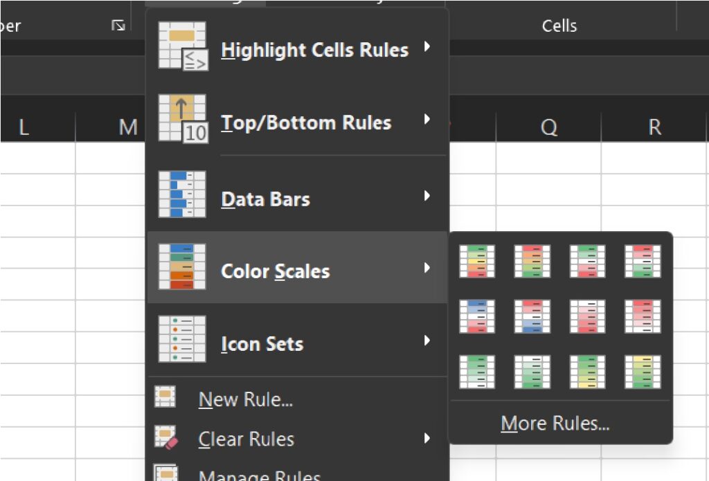
• Choose the cell range.
• Go to the Styles Group > Conditional Formatting section on the Home tab.
• Choose a subtype by clicking Color Scales.

Icon sets in conditional formatting

Shapes, arrows, check marks, and other objects are used in Excel Conditional Formatting icon sets to help display the data. The steps below can be used to add an icon set:

You can utilise built-in icon sets for conditional formatting in Excel and subsequent versions. These icon sets offer a quick way to distinguish between a list of numbers’ high, medium, and low values.

Shapes in the typical shades of green, red, and yellow are used in many icon sets. Some icon sets come in alternative colour schemes, such all-gray or black and white.

• Choose the cell range.
• Go to the Styles Group > Conditional Formatting section on the Home tab.
• In the Icon Sets window, click a subtype.
• Go to Conditional Formatting > Manage Rules > Edit rules to make changes to the rules. To suit your preferences, you can alter the rules.

Delete conditional formatting rule

When required to remove a conditional formatting rule you’ve created later. There are two ways to delete a rule, and the procedures are as follows:.

• Go to conditional formatting dialog box-> Clear rules
• The entire sheet, or just the conditional formatting rules in certain cells, can be deleted.
• Alternately, you can remove a specific set of conditional formatting rules from a sheet’s selected cells or from all of them.

Delete all rules

Use the instructions below to delete all conditional formatting rules from a specific cell or the entire sheet.

• Choose the cells you wish to remove ALL the rules from.
• Alternatively, if you wish to remove all rules from the current page, choose any cell on the worksheet.
• Click the Home tab on the Excel Ribbon.
• Click the Conditional Formatting command in the Styles group.
• Next, select Clear Rules at the bottom of the list of choices.
• Select one of the choices:
• Either clear the rules from the selected cells or the entire sheet.

Delete specific rules

These steps should be followed to select rules in the Conditional Formatting Rules Manager in order to eliminate a particular rule:

• Choose the cells B2 through E7 where the initial conditional formatting rule was used.
• Click the Home tab on the Excel Ribbon.
• Click the Conditional Formatting command in the Styles group.
• Next, select Manage Rules from the options list at the bottom.

Conditional formatting rules

Microsoft Excel’s conditional formatting rules management window

The Conditional Formatting Rules Manager window contains a wealth of data and features. Let’s examine the various components of the window.

Current Selection is the list’s default entry under “Show formatting rules for.” Because we clicked a cell within the formatted range, both rules are visible.

To view every rule for a certain sheet, edit this list. Finding the Conditional Formatting rules on a sheet is made much easier by using this.

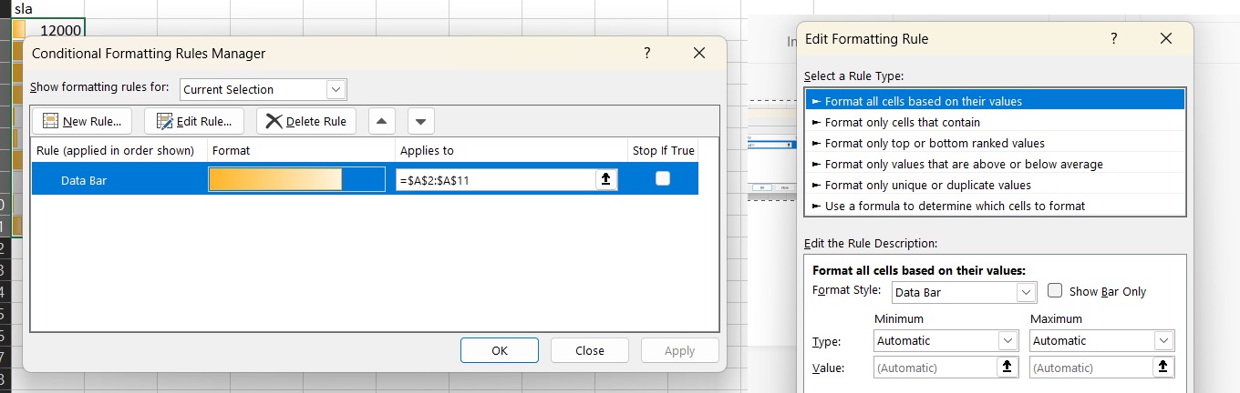
The rules are provided with columns for the format, range, and applicable rules.

• To create, amend, delete, and duplicate rules, use the buttons.
• Change the order of the rules using the two up/down arrows next to the buttons.
• Both styles are used when more than one rule is True, with the rule at the top of the list being applied last.

In Microsoft Excel, the “Edit formatting rule” panel was used to apply various formatting rules to data bars.

Conclusion

Some of our best Excel Instructor in Delhi tried to explain conditional formating in Excel in a very comprehensive way through this article. If you want to further take a Advanxce Excel Course from best Excel Institute in Delhi,