
We utilize the VLOOKUP and HLOOKUP function when we need to search through a large spreadsheet for information or when we frequently need the same kind of data.
Use: As a technique of chopping and dicing data for analysis, LOOKUP and similar functions are frequently employed in Excel’s business analytics.
In simple, its syntax includes 4 arguments:
=VLOOKUP(Value, Table, Col. Index no. ,[Range Lookup]) OR
=HLOOKUP(Value, Table, Row Index no. ,[Range Lookup])
Lookup value: This is the value that has to be found in a table’s first column.
Table: The table from which the value is fetched is indicated by this.
index no. : The table column/row from which the value should be obtained.
Range Lookup: TRUE = roughly match (default). EXACT MATCH = FALSE
But what if I said that V/H Lookup is capable of much more? You can utilize it in numerous ways with the same syntax rather than just concluding by speaking a line about it.
That implies that you will only be doing VLOOKUPs but in various situations that you thought were so hectic to perform manually or standard processing. Let’s discuss….
Common Use Cases for Vlookup in Microsoft Excel
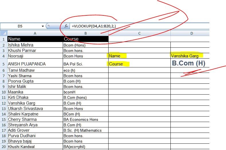
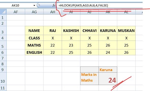
NORMAL VLOOKUP/HLOOKUP
It’s the normal VLOOKUP/HLOOKUP that you would have performed or being performing in your classes i.e. from the same sheet. This means all the data and the resultant sheet is in the similar sheet. This can be simply done by applying the syntax highlighted above.
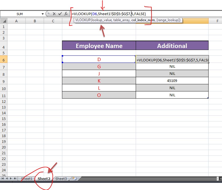
VLOOKUP/ HLOOKUP FROM DIFFERENT SHEETS
Here, you can perform VLOOKUP/HLOOKUP with required data and the resultant is on different sheets. Like, suppose you have a record and you have to copy of some or collect of some for analyzation purpose, then also you can do it with the help of these LOOKUP functions. Your work of looking through that lengthy list for the names and sales targets will be eliminated.
SYNTAX: = VLOOKUP(lookup_value, Table_array, Index_no.,[Range Lookup])
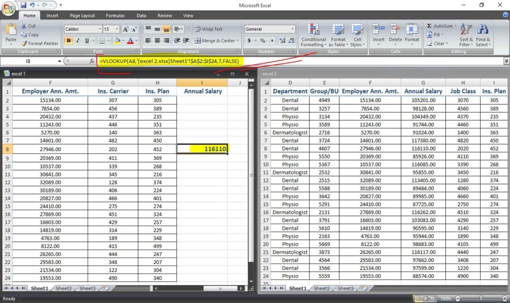
You can even do it from different workbooks by just focusing on what array should be selected.
COPYING VLOOKUP FORMULA
Since, it’s easy to drag and copy the formula vertically down but the situation is not same when we talk about horizontal copy paste. Whereas, while working we have to use both to manage time and tasks in an efficient manner. So just have a look how we can do it horizontally as well.
Step 1. Go to the cell where you want the outcome and type syntax and press ENTER.
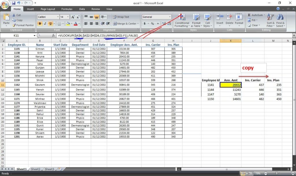
Step 2. Copy horizontally i.e. to fill up the row information
Step 3. Modify the syntax by keeping the Lookup Value unfixed while rest of the formula stays same as above and press ENTER.
Step 4. Copy down vertically.
Is it necessary to unfix the lookup value before copying vertically and fixing it for copying it horizontally?
Ans. Yes , it is. Because fixing the lookup value won’t allow the function to use values listed down as lookup value while copying and all the outcomes will be from the same lookup value instead of their respective lookup values. Whereas, while copying horizontally , it is necessary to block the lookup value because needed outcomes are for the same lookup value.
TO FIND MULTIPLE MATCHES
Sometimes, like in a list of sales we can have a same client many times, So, what if I have to find how many times I made sales to him? Should I start to count from the top and sit till the end? No. Not at all. Here I will use Lookup Function to list the same company sales together for analysis.
SYNTAX:
=VLOOKUP(Lookup_value & Row()- n,Table_array, Match(lookup_value,lookup_array,[match_type], Range_Lookup)
Here, we want a dynamic outcome, therefore we’ve added an operation that could provide us with various row cells depending on what we need. And from the row we are now in, we must deduct the necessary number of rows in order to get to the first cell that contains the lookup value. For example, if we are entering the formula in row 10 and we are starting from cell B3, or row = 3, we will enter ROW()-7 to get to 3.
Step 1. First of all, get the occurrences ranked using the formula given below:
SYNTAX: =cell_ref & COUNTIF(cell range,criteria)
Step 2: Type the lookup syntax mentioned above in the cell where you want the outcome and press ENTER.
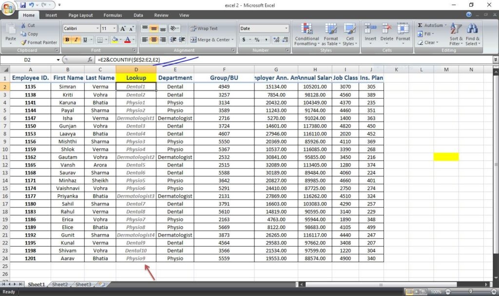
Step 3: Copy it the whole array.
Altering the data in cell containing lookup value will automatically alter the resultant outcomes.
NOTE:
- Ranking the occurrences is an important step and can’t be eliminated.
- Headers should be same in the array and at the destination of the outcomes to work with MATCH function.
TO COMPARE TWO LISTS
Sometimes, like in companies, different registers are maintained along with different levels. And sometimes due to some discrepancies, the data differs. But is it easy to match those datasets and records manually? No. It would interest you to know that you can do this by using Lookup Functions. Here is an example of Vlookup but you can follow the same steps with Hlookup.
SYNTAX: =IF(ISNA(VLOOKUP(Lookup Value, Table Array, Column index no.,[Range Lookup])),[value if true],[value if false])
We have attempted to cover all potential uses for the Vlookup and Hlookup functions. It would be impossible to include them all because these functions can be combined with several other functions to provide dynamic results. But I made an effort to include at least some of the fundamentals that any Excel user should be familiar with. Learn more and succeed at it.
Do you want to pursue a complete Advance Excel Course from best excel institute in Delhi? Enroll now