
Do you know mastering Excel formulas can be a very good step to in becoming a Data Analyst? Well, the reputed faculty trainers from one of the best Computer Training Institute are sharing their insights on the most important excel formulas one should know. Excel formulae, with a little practice, makes you an expert at it in no time. The article itself is like a Free Excel Course for beginners.
What is Excel?
The Microsoft Office suite of business applications includes the spreadsheet tool Excel. Users of Microsoft Excel can format, arrange, and compute data in a spreadsheet. It is typically used to provide data reports and business insights that can be quickly and readily interpreted.
Why to use Excel?
Basically, it’s used to show and evaluate financial or business data. Utilizing pivot tables, graphing tools, and numerous built-in apps, users can arrange their data to make it more presentable and feasible to analyze. The main uses of excel includes:
- Data entry
- Data management
- Accounting
- Financial analysis
- Charting and graphing
- Programming
- Time management
- Task management
- Financial modeling
- Customer relationship management (CRM)
What are Formulae in Excel?
Among all the built-in capabilities, Excel sheet formulas are one that helps Excel to stick out.
A formula in Microsoft Excel is an expression that modifies values in a set of cells. It is used to do mathematical calculations without having to exert much mental effort. You may execute calculations like addition, subtraction, multiplication, and division using Excel formulae. Excel also allows you to work with date and time values, discover averages and percentages for a range of cells, and perform a lot more things.
- Two distinct concepts: Formulas and Functions
Even though they sound similar and they might have been used as a substitute for one another, but actually, they are not. A Formula in Excel is an equation created by the user, whereas a Function is a predetermined computation in the spreadsheet application.
Formula: Here, we operate on values of a cell or range of cells.
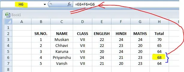
Like, in the image 1, for getting the total of Priyanshu’s marks, values in a range of cells are operated with the arithmetic sign ‘+’ i.e. E6+F6+G6.
Function: Here, to ease our work some functions are predefined and it eliminates our efforts of applying the operational formulae gain and again.
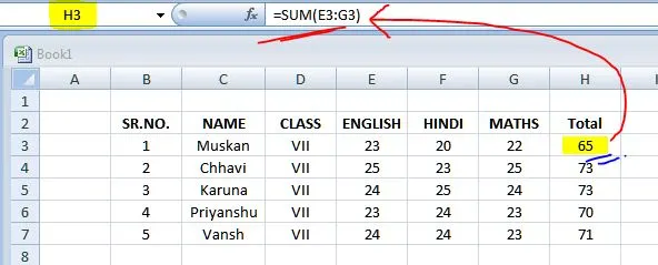
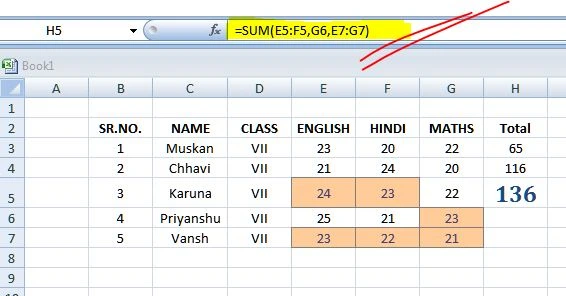
Like, in the Image 2, for getting the total of Muskan’s marks, instead of using ‘+’ again and again along with the individual cell addresses, the function ‘SUM’ is used ; i.e. =SUM(E3:G3)
Fig.2: Microsoft Excel Function
Formula/ Function Insertion Methods in Excel
Although entering the formula straight into the cell is the most commonly used approach, there are several ways to insert formulas. Let’s have a look on them also;
- Typing the formula directly inside the cell
Inserting the formula straight into the cell we want result is the most common way
Excel is quite sophisticated in that it will display a function hint when you begin typing the name of the function
However, when you’ve made your pick, don’t press the Enter key. Instead, use the Tab key to have Excel fill in the function name for you.
- Typing the formula in formula bar
- Left-click the cell in which you want your result to come
- Enter the formula in the formula bar above
- Press Enter
- Using Insert Function option from Formula Tab
- Left-click the cell you want result to come in.
- Go on Formula Tab and choose the Insert Function option.
- A dialog box will appear. Now you have 2 ways to deal:
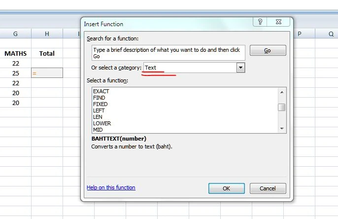
Just enter the name of the function you want in the Search for a function Box and press GO button. Your preferable function will be automatically highlighted in Select a function sliding list
Select the category you want from the drop-down list, like, we chose the category ‘TEXT”. So, all the options related to Text manipulations only are shown in select a function list. Choose the one you want and click OK
Function Arguments dialog box will appear.
Here, you must enter the range of cells you need for calculating. Or else, if you want to type the particular numbers you want to do operations with, then you can directly type the number, like, the first number in Number 1 column, second one in Number 2 column and so on.
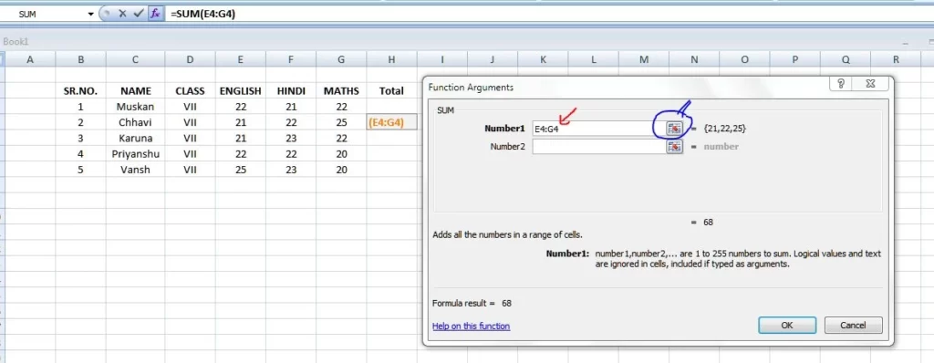
Alter the range of cells by clicking on the button marked with blue and press Enter.
- Selecting a Formula from one of the Groups of Formula Tab
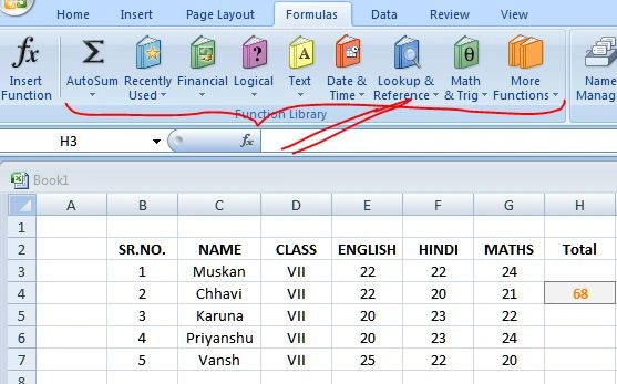
Navigate to the Formulas tab and pick your favorite group to access this menu. Click to reveal a sub-menu with a list of functions. You can then choose your preference. If your favorite group isn’t on the tab, choose the More
Formulas & Functions of Microsoft Excel
Excel formulae and functions abound. We’ll go over the formulae and functions that any Excel newbie should be familiar with. They are:
Mathematical Functions
- Sum: It Adds Value
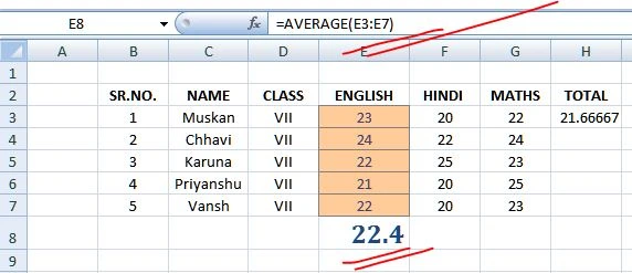
- Average: It calculates the averages of the data
Syntax: =AVERAGE(no.1,no.2,no.3,…) or =AVERAGE(Range of Cells) and press Enter.
- MAX: It returns the maximum value in the data provided.
Syntax: =MAX(no.1,no.2,…) or =MAX(range of cells)

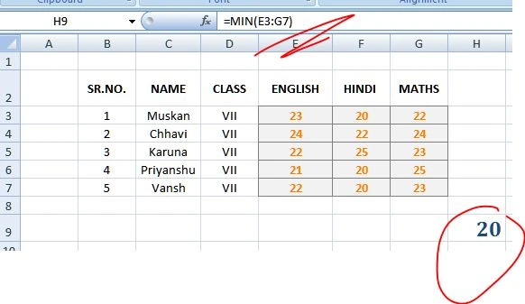
- MIN: It returns the minimum value in the data provided.
Syntax: =MIN(no.1,no.2,.. or range of cells
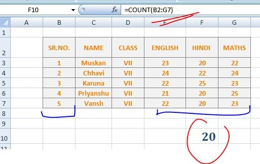
- COUNT: Count the cells with Numbers.
Syntax: =COUNT(value1,value2,.. or range of cells)
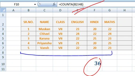
- COUNTA: Count the cells that are not blank.
Syntax: =COUNTA(value1,value2,.. or range of cells)
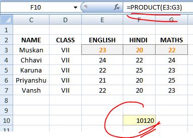
- Product: It returns you the product of the values selected
Syntax: =PRODUCT(value1,value2,.. or range of cells)
Text Functions
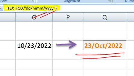
- TEXT: By applying formatting to a number using format codes, the TEXT function enables you to alter how it appears
Syntax: =TEXT(Value you want to format, "Format code you want to apply")
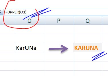
- UPPER: It returns the text of the selected cell in upper case.
Syntax:=UPPER(text)
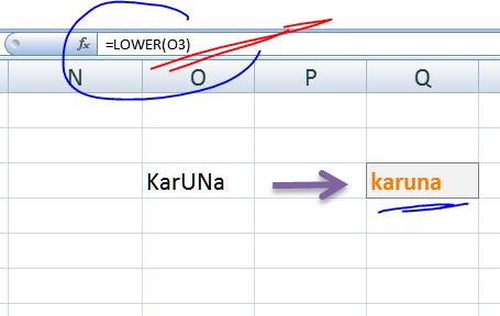
- LOWER: It returns the text of the selected cell in lower case.(See Fig. 23)
Syntax: =LOWER(Text)
- PROPER: It returns the text in the sentence case.
Syntax: PROPER(Text)
- RIGHT: It returns the right-hand side characters from a textstring. (See Fig.25)
Syntax: =RIGHT(text,[num_chars])
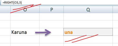
Fig.25
- LEFT: It returns the left-hand side characters from a textstring
Syntax: =LEFT(text,[num_chars])
- MID: Based on the user-specified beginning position and character count, Excel’s MID function returns the number of characters from a text string
Syntax: =MID (text, start_num, num_chars)
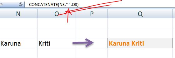
- Concatenate: It can be used to connect text fragments together or combine values from many cells into a single cell.
Syntax:=CONCATENATE (Text1,Text2,,,,) or =CONCATENATE(text1,” “,text2) if space needed
- LEN: It gives you the number of letters, numbers, characters and spaces in the cell selected.
Syntax: =LEN(Text)
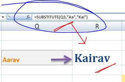
- SUBSTITUTE: It is used to replace any portion of an old text string with a new text string.
Syntax: =SUBSTITUTE(text, old_text, new_text, [instance_num])
*instance num: If you specify instance_num, only that instance of old_text is replaced. Otherwise, every occurrence of old_text in text is changed to new_text.
- REPLACE: The Excel REPLACE function swaps out characters in a text string specified by location with characters in another text string.
Syntax: =REPLACE(old_text, start_num, num_chars, new_text)
- TRIM: With the exception of the single spaces between words, Excel’s TRIM function removes all irregular spaces from the text.
Syntax: =TRIM(Text)
Date and Time Functions
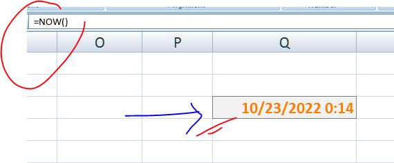
- NOW: It Displays the current date and time.
Syntax: =NOW()
- DATE: returns a serial number of a date based on the year, month and day values that you specify.
Syntax: =DATE(year,month,day)
- DAY: returns the day of the month
Syntax:=DAY(Serial number)
- MONTH: returns the month of a specified date
Syntax: =MONTH(Serial number)
- YEAR: returns the year of a specified date
Syntax: =YEAR(Serial Number)
- TODAY: returns today’s date
Syntax: =TODAY()
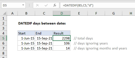
- DATEDIF: returns the difference between two dates
Syntax: =DATEDIF(start_date, end_date, unit)
- HOUR: Returns the hour of a time value
Syntax: =HOUR(serial_number)
- MINUTE: Returns the minutes of a time value
Syntax:= MINUTE(serial_number)
- SECOND: Returns the seconds of a time value
Syntax: =SECOND(serial_number)
Lookup Functions
- VLOOKUP: This is an acronym for the vertical lookup, which searches the leftmost column in a table for a specific value. It then returns a value from the specified column in the same row
Syntax: =VLOOKUP(lookup value,array,col_index_num,range lookup)
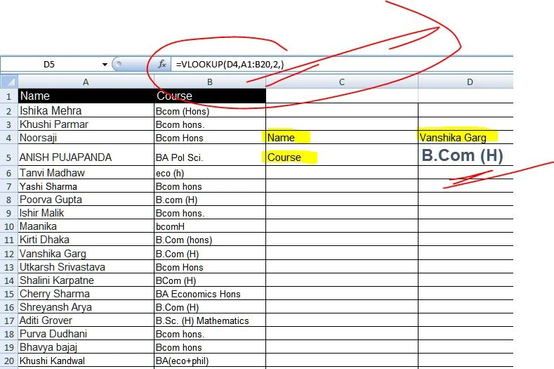
Lookup value: This is the value that has to be found in a table’s first column.
Table – The table from which the value is fetched is indicated by this.
Col index – The table column from which the value should be obtained. [Optional] Range lookup: TRUE = roughly match (default). EXACT MATCH = FALSE
- HLOOKUP: The function HLOOKUP looks for a value in the top row of a table or array of benefits. It gives the value in the same column from a row you specify.
Syntax: =HLOOKUP(lookup value,array,row_index_num,range lookup)
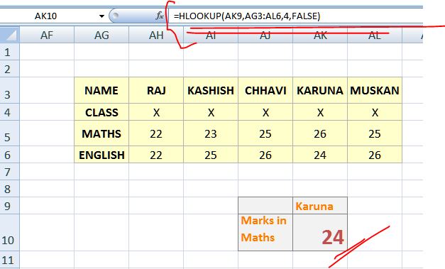
Lookup value – The value to lookup is indicated by this.
Table: The table from which you must retrieve data
Row index is the row number that should be used to get data.
[Optional] Range lookup: This boolean value represents an exact or approximative match. The default value, TRUE, denotes a close match.
- TRANSPOSE: It is used to switch or rotate cells
Syntax: =TRANSPOSE(Array)
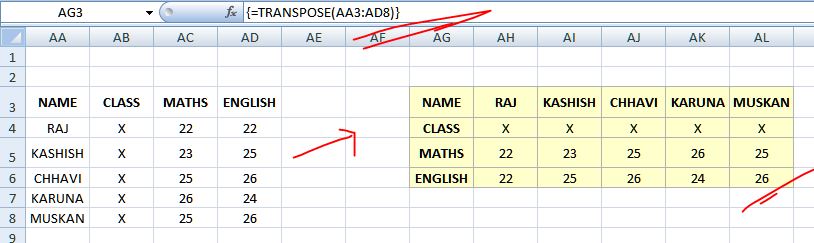
After entering the formula, you need to press Ctrl+Shift+Enter instead of just Enter.
Types of Errors in Microsoft Excel
The sole automatic calculation capability in MS Excel that is widely used is what we can accomplish by using a variety of functions and formulae. But when we use formulas in an Excel cell, we get many kinds of errors.
The list of 9 top and common errors are:
- #DIV/0!: When we use a formula in a spreadsheet to divide two numbers and the divisor (the number being divided by) is zero, we get an error. It is an abbreviation for divide by zero mistake
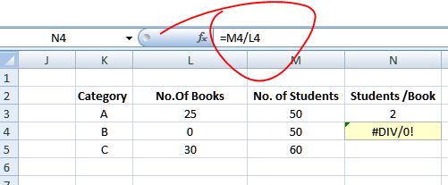
Solution: Use ‘IF’ Function instead
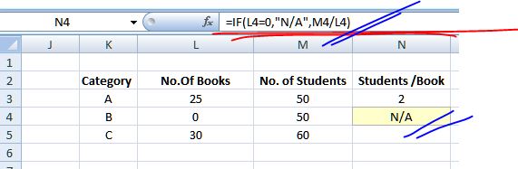
- #N/A “No value available” or “not available”. It means that the formula is unable to locate the value that we had assumed it would
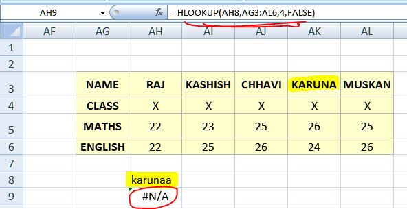
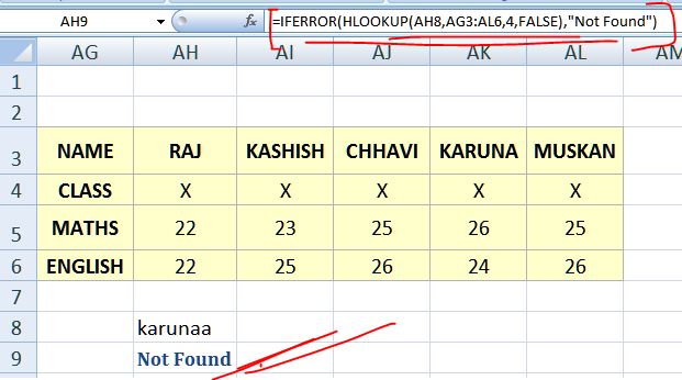
In the table ‘Karuna’ is written with this spelling, whereas, in formula the cell selected has ‘karunaa’, that’s why, it showed an error. Solution: Use of IFERROR. It would eliminate the display of #N/A error and would display the text you will be willing to show like, Not found, Nil etc
- #NAME: When we typically misspell the function name, this error is shown
Solution: Rectify the Name of the Function
- #NUM!: Invalid numbers for any function argument will typically result in the display of this error. Like if you are finding the Square roots or cube roots of a negative number or you are using numbers that are either beyond or not within the limits of numbers the excel spreadsheet allows.
Solution: Correct the number as per mathematical or excel rules and limits. Like here, we need to make it positive .i.e. 5 instead of -5.
- #REF!
Reference error is what this error means. This error typically occurs when
- Our formula’s reference cell was mistakenly erased (see Fig.55)
- The linked cell is copied and pasted in several places.
Solution: Try not to remove or move the referenced cell.
- #####: When the column width in Excel is insufficient to display the value recorded in the cell, this error is shown
Solution: Adjust the size of the cell according to the data.
- Circular reference: This mistake occurs when we use the same cell reference as the one where the function or formula is being written
Solution: Be careful while selecting the range of cells for computation.
- #VALUE!: The improper data type is used in a function or formula, which results in this error. Like, if unintentionally, you add up texts instead of values (see fIg.56)
Note: Adding up texts by applying SUM function will end up with Zero ‘0’. This would appear only if you use formulae.
CONCLUSION
Given Excel’s great popularity, there are probably only a small number of people who haven’t used it. In today’s sectors, Excel is a software programme that is frequently utilized. So, everyone should have at least basic knowledge of Microsoft Excel.
Without a doubt, having a solid understanding of Excel helps to shape numerous vocations. For data analysis and reporting, Excel is a fairly strong spreadsheet programme. We examined complex Excel formulas and functions, text, data-time, and numeric formulas. After reading this article, perhaps you now have a better understanding of the key Excel formulae and functions that will enable you to do your duties more quickly and effectively.
Looking for a proper Microsoft Excel Course with Hands on training online or offline? ESS Institute, Being a top computer Institute of Delhi located near Dwarka mor has a special Computer course for Microsoft excel, word and basic computers