Every material thing in the universe is defined by space and time. The efficiency of an algorithm can also be determined by space and time complexity. Even if there are many methods to approach a particular programming challenge, understanding how an algorithm operates could help us become better programmers. Time complexity is suggested to be a key metric for measuring how well data structures and algorithm’s function. It gives us a sense of how a data structure or algorithm will function as the volume of the input data increases. Writing scalable and efficient code, which is crucial in data-driven applications, requires an understanding of time complexity. We will examine time complexity in Python data structures in more detail in this blogpost. Let’s go through it.
What is Time Complexity in Python?
In computer science, the phrase “time complexity” refers to the computational complexity which we can use to characterize how long it takes for an algorithm to run. Counting how many basic operations the algorithm does, given that each basic operation takes a specific amount of time to complete.
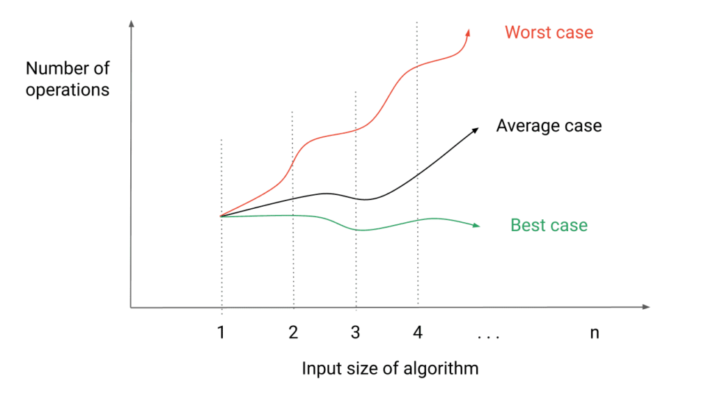
Generally we have 3 cases in time complexity
- Best case: Minimum time required
- Average case: Average time required
- Worst case: Maximum time it need to compute
It’s is a standard method for estimating time complexity. It’s usually expressed in big-O notation, which represents the upper bound of the worst-case scenario. Big-O notation helps us to compare the performance of different algorithms and data structures in terms of their scalability.
Python counts the number of operations a data structure or method needs to perform in order to take a given task to end. Data structures in Python can have a variety of time complexity, including:
1. O(1) – Constant Time Complexity: This denotes that the amount of time required to complete an operation is constant and independent of the amount of input data. For example: When we access an element in an array by index, it has an O(1) time complexity. because the time required to access an element is constant regardless of the size of the array.
2. (log n) – Logarithmic Time Complexity: OThis describes how the time required to complete an operation grows exponentially with the size of the input data. For example, Since the search time increases exponentially with the number of items in the tree, a binary search tree has a temporal complexity of O(log n) when looking for an element.
3. O(n) – Linear Time Complexity: This specifies that as the size of the input data increases, the time required to complete an operation climbs linearly. As an example, running algorithm over an array or linked list is having time complexity of O(n) because the amount of time needed to run over each member grows linearly as the size of the array or linked list does. Due to which iterating over them has an O(n) time complexity.
4. O (n log n) – Log-Linear Time Complexity: This describes how an operation’s time complexity is a blend of linear and logarithmic. As an example, the time complexity of sorting an array with a merge sort is O(n log n). It is Because of the time needed to divide and merge the array grows logarithmically while the time needed to compare and merge each element grows linearly.
5. O(n2) – Quadratic Time Complexity: This refers to the fact that as the size of the input data increases, an operation’s execution time climbs quadratically. For instance, sorting an array using bubble sort has an O(n^2) time complexity because it takes more time to compare and swap each element as the array gets larger.
6. O(2^n) – Exponential Time Complexity: This refers to the fact that as the size of the input data increases, same will gonna happen with the time required to complete an operation. For instance, because the number of subsets grows exponentially with the size of the set, creating all conceivable subsets of a set using recursion has a temporal complexity of O(2n).
7. Factorial time (n!): When every possible combination of a collection is calculated during a single operation, an algorithm is said to have a factorial time complexity. As a result, the time required to complete a single operation is factorial of the collection’s item size. The Traveling Salesman Problem and the Heap’s algorithm (which creates every combination of n objects imaginable) are both O(n!) time tough problems. Its slowness is an issue.
Python data structures’ time complexity must be understood in order to write scalable and effective code, especially for applications that work with big volumes of data. We can enhance the performance and efficiency of our code by selecting the proper data structure and algorithm with the best time complexity.

Why do we need to know time complexity of data structures?
We can optimize our code for effectiveness and scalability by knowing time complexity, which is crucial when working with large data sets. We can decide which strategy to use to solve an issue based on the time complexity of a specific algorithm or data structure in Python. When we kook out\ for an element in a huge dataset, we might go for a hash table rather than an array because the time complexity of a hash table search is O(1) as opposed to O(n) for an array. When processing a lot of data, this improvement can help us save a lot of time. Additionally, it helps us stay clear of programming errors like nested loops and recursive functions, which can cause extremely slow execution.
Common Time Complexities in Data Structures
Time Complexities of Array in Python
Arrays are a basic data structure that let us efficiently store and access components of the same type. Python implements arrays as lists, and the following operations have the following temporal complexity.
1) O(1) for accessing an element by index
2) Adding an element at the start: O(n)
3) Adding a component at the end: O(1)
4)Removing a component at the start: O(n)
5) Removing a component at the conclusion: O(1)
Time Complexity of Linked Lists
Linked Lists are Another basic data structure which are made up of a series of nodes, each of which has information and a link to the node after it. The use of classes and objects allows us to implement linked lists in Python. Following are some operations with a high temporal complexity.
1) When accessing an element via its index O(n)
2) Inserting an element at the beginning: O(1)
3) Adding a last element: O(n)
4) Removing an element at the beginning: O(1)
5) For removing a component at the conclusion O(n)
Time complexity of Stack
Linear data structures that adhere to the Last-In-First-Out (LIFO) concept include stacks. Lists can be used to implement stacks in Python. The following operations have a high temporal complexity:
1) O(1) for adding an element to the stack.
2) O(1) for popping an element from the stack
3) Getting to the first element: O(1)
Time complexity of Queues
A queue is a type of linear data structure that follows the First-In-First-Out (FIFO) principle. In Python, we can also implement queues using lists. The time complexity of common operations is as follows:
1) Enqueuing an element: O(1)
2) Dequeuing an element: O(1)
3) Accessing the front element: O(1)
Time complexity of Hash Tables
A hash table is categorized as a type of data structure that enables key-value pair-based data storage and retrieval. Hash tables can be created in Python by using dictionaries. The following operations have a high temporal complexity.
1) Accessing an element by key: O(1)
2) Inserting an element: O(1)
3) Removing an element: O(1)
Conclusion
For creating code that is effective and scalable, it is crucial to comprehend the time complexity in data structures. For typical tasks, Python offers us a variety of built-in data structures with varying time complexity. If we Know the temporal complexity of each data structure, it will allow us to select the best one for our application and will going to speed up our code. The main operations of Python data structures were described in this article using Big-O notation. In essence, the big-o notation is a technique to gauge how time-consuming an operation is. A number of typical operations for a list, set, and dictionary were also shown in the article.
How the programs use space and time efficiently is the key difference between an average python programmaer and a good python programmer. A good Python programmer will always end up with better packages than just a programmar,If you want to cross that line to become a good coder, you need to learn python from professionals, join ESS institute now to learn from the Best Python institute in Delhi
You can also join our online Python course now. Vist ESS Computer Institute in Delhi to know more about is